Background – Over past few years we have implemented IBP Order Based Planning Deployment optimizer for few customers mainly in Consumer goods industries where goods flow and Supply chain networks are complex , during implementation we have faced lot of challenges/hurdles. In this blog, we are trying to provide some insights to those challenges which we have faced while implementing OBP deployment optimizer. For lot of these topics we have worked very closely to give them a good shape and make them usable for customers. Without wasting much time lets get into the details and see what all was done during our journey.

1. Optimizer log vs Planning view mismatch (Bucket level vs Time continuous planning)

Overall Order based planning framework is based on time continuous planning and Optimizer engine works on bucket level planning, so below step happens when you take OBP Deployment optimizer run

• Aggregation of time continuous data at bucket level to prepare input for optimizer
• Optimizer plans at bucket level and generate output at bucket level
• Optimizer output is converted into time continuous data using post processing step. Optimizer output does not result in direct creation of orders rather the output is passed on as instructions to a post processing step which actually creates these orders and also generates pegging

Due to different concepts, if your Available to deploy qty (like Process/Production/Planned orders) are available with time stamp other 00:00 hours then we see the mismatch between what optimizer has planned and what output has been created as orders in planning view. To minimize such mismatch there are 2 possible solutions :

• Bring all the receipts (Like Process/Production/Planned orders) at 00:00 time stamp which is actually start of the bucket
• SAP has additional parameter to manage this issue without making any change in time stamp of incoming receipt data.

2. Demand Unfulfillment

Generating demand unfulfillment information is key factor to analyze deployment output, generate alerts and have correct projected stock and coverage, there are standard settings available in OBP Planning run profile

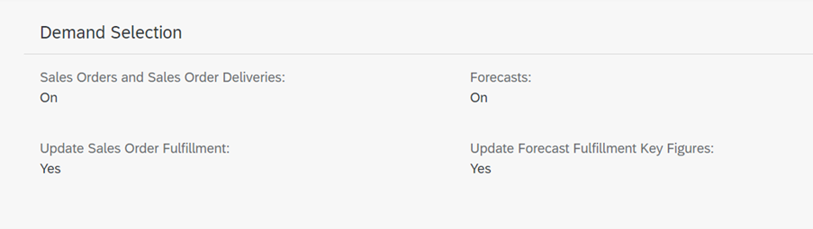
Apart from that we also have good number of KF to provide this information (others are generated based on pegging created in post processing step.

Please note depending on your scenario you would have to include some of these key figures manually in your Total Demand, Projected Stock calculation to have right information, these are not by default included in Total Demand or Projected Stock calculation in SAP7(F) design.

3. Modelling Stock under Quarantine

In standard OBP its not possible to model the stock which is produced but lying under quarantine, this kind of stock is normally available in form of batch restricted stock and is critical to be planned properly with Deployment. As this is not visible on OBP side the engine is not able to plan this stock upon its availability. As a workaround its possible to model this stock as future dated receipt/order in ECC or S/4 by doing a development in the available Stock and Order BADI.

Note that this is a very complex development and proper assessment should be made before trying this approach.

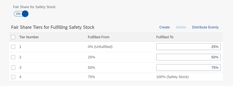
4. Safety stock modelling (Days Vs Qty)

This is a design element which is always discussed in every project, while planners are used to work with days as it provides simplicity on the other side most of the Inventory optimization algorithm would provide their output in pure safety stock numbers.

Now coming to OBP deployment optimizer, we can also model both safety stock days or qty but if we are using fair share functionality and would like to have a proper fair share across your supply chain network then we strongly suggest you to use Safety stock as quantity. There are serious limitations if you use Deployment optimizer with Safety days and this can make the output look very bad.

You can calculate safety stock qty beforehand and then pass it to optimizer as an input. One of an easy way is to utilize IBP_COVERAGE() function and then convert Safety stock days to Safety stock qty, you would have to make sure that you calculate your demand properly in order to have proper safety stock numbers. Final remark if you are working with Safety stock quantity then you might have to make a comprise in considering your distribution demand as this is normally an output of the planning algorithm, in such scenarios you might have to include distribution demand from a previous run or do some rough cut calculation.

5. Fair share (Linear and Non-linear)

Fair share of stock and demand is a crucial requirement for many of the clients who have dynamic Supply chain network and changing Demand/Stock situation on day to day basis. Overall, in IBP OBP Optimizer we have following fair share options available :

• Demand Fair share

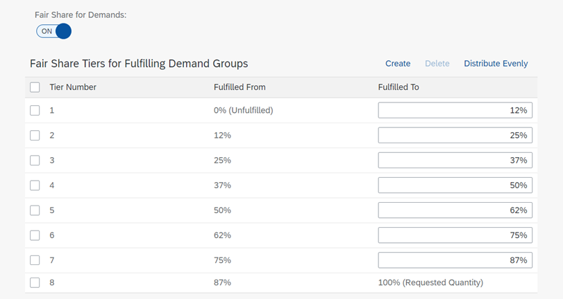
• Safety stock Fair share

• Max stock Fair share

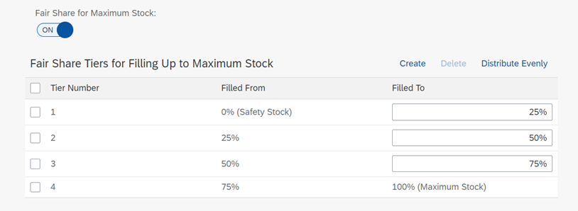
• Excess Stock Fair share

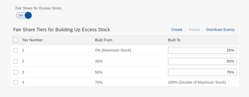
Please note that tiers can be defined with linear / non-linear distribution it ranges between 2 to10 but in standard cost distribution always varies on linear basis.

Overall, 10% cost increase applies for all the tiers, so if we have 4 tiers then every tier will get the cost increase of 2.5%. Its very important to understand that In case of stock fair share its further divided on equal basis between segments defined on Location Product master data level in ECC or S/4. You can also assign same segment to all the location product to make it simple.

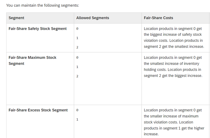
In case you want to have much more increase in costs for different tiers then SAP with their expert consulting services can help provide you additional parameter(s), please note that the standard cost increase is 10% across tiers.

For more information about OBP Fair share, please read SAP Help

Non-linear cost distribution is also possible, SAP has additional parameters to achieve the same but it makes solutions complex and increases number ranges / cost variations so it’s not recommended to go for non-linear cost distributions.

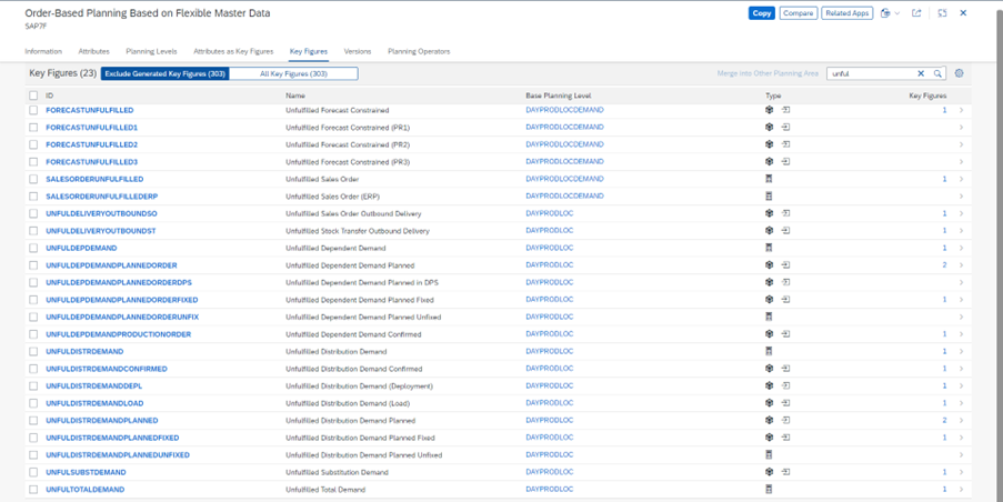
6. Projected Stock and Days of Supply Calculation

Although standard SAP7(F) provides two standard key figures for the same (STOCKPROJECTED and DAYSOFSUPPLY) but standard KF STOCKPROJECTED does not factor unfulfilled demand KF so it doesn’t provide what is the real Projected Stock on hand.

For proper analysis we need to create a new custom key figure Stock Projected ATD which is calculated as (STOCKPROJECTED – UNFULFILLEDDEMAND), this KF can then be used to calculate another custom KF which is Days of Supply ATD.

7. Stock Coverage %

Depending upon which fair share we are analyzing (Safety stock, Maximum stock or Excess stock), we need to create corresponding Stock Coverage or Stock Level % key figure so we can see how if the stock distribution is happening in fair share way or not

• Safety stock Fair share Stock Coverage % = (Stock Projected ATD / Safety stock) * 100
• Max stock Fair share Stock Coverage % = ((Stock Projected ATD – Safety stock) / (Maximum Stock – Safety stock)) *100
• Excess Stock Fair Share Coverage % = ((Stock Projected ATD – Maximum stock) / (2*Maximum Stock)) *100

8. Safety stock violation cost (weekend behavior)

Basic prerequisite for fair-share to work that all the parameters including costs should be maintained in a fair way. In our scenario we had receiving / shipping calendar as five days working (most of the Plants/warehouses operating during weekdays only) but we had safety stock and violation costs definer over weekend too. Because of this fact optimizer in lot of circumstances was trying to push stock to destination location near/before weekend as it was saving the safety stock penalties which it would normally occur on weekend.

This is not desirable from planner perspective as in real life you would normally receive that stock after weekend. To resolve this issue we are now modelling safety stock and its violation cost only on working days, post this change we have seen significant improvement in the results.

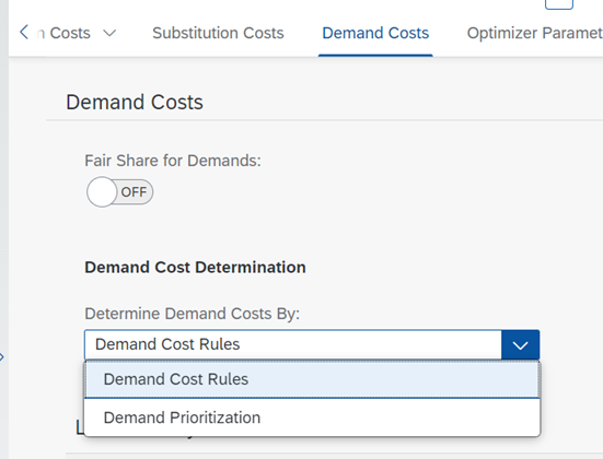
9. Demand cost modelling (Demand Rule vs Cost Rule)

We can generate Non Delivery cost by two ways, there are specific options in planning run by which you can define how non delivery cost rates will be calculated. Below two are the options available :

• Using Demand prioritization rules
• Using Demand cost rules

10. Transportation Resource Modelling (Unavailability of Non-Delivery cost rate as key figure)

Currently Non delivery and Late delivery cost maintenance area only available via Planning run profile as cost rules and not available as KF. Because of this fact that we couldn’t model Transportation resource as constraint because it requires to maintain Non delivery cost in one common UOM which can only be done at KF level.

So, if you are thinking of using Transportation Resource as a constraint please be aware of this limitation, also there are no roadmap items to have both Non Delivery and Late Delivery available as key figures in OBP although they are available as key figures in Time-series.

11. Demand discount factor in OBP

A very common requirement to prioritize bucket “X” demand over “X+1” is Demand discount factor, happy news is that Demand discount factor is supported and built by default in Order based planning optimizer.

The demand discount factor is internally hardcoded and applied based on your planning horizon, the engine will automatically apply a difference of 10% between the first bucket and last bucket using linear function. So, if first bucket cost is 1000 then second bucket cost will be 990 and last bucket cost will be 900.

12. Deployment Auto cost generation

Although Deployment optimizer has auto cost generation option (similar to APO Auto Cost Generation) but based on our tests we haven’t found it much useful so we suggest to create your own cost model and don’t use auto cost generation functionality.

Please note that this is our suggestion based on the tests we have done, you must depending on your business scenarios and models must decide if you should use it or not.

13. Transport holding cost policy

In order to generate meaningful Deployment stock transfer, there is a setting available in planning run profile but we strongly suggest not to use this setting instead discuss with SAP to use the additional parameter related with transport cost holding policy.

14. Cyclic lane

A typical scenario which you may see are the cyclic lanes in the network. Although optimiser is capable to handle cyclic lanes (with relevant transportation cost) but we had seen lot of issues during post processing/order creation step. We have resolved all these issues by applying some expert parameters after discussion with SAP.

One very typical issue which we have seen in case of cycles are creation of standard STRs (not type Deployment), this issue can again be solved by applying expert parameters.

15. Modifying deployment plan (Manual adjustment)

A typical function in planner life is to modify the deployment plan on day to day basis to reflect business needs. Now when it comes to changing the Deployment plan in OBP there are three ways and each of them will have their own challenges :

• Manually creating orders from Projected Stock app – its very time consuming as it allows to create order by order. No mass creation of order possible from here
• Using Interactive KF – this creates new orders only whenever we run the application and existing orders cannot be changed. We need to keep deleting interactive KF values to avoid multiple order creation
• Min/Max Distribution key figures – we need to maintain this key figure and take deployment planning run to consider these values. After converting deployment STR into STO, one needs to remember to clear the values min/max key figure otherwise it will generate new STR again

Moving forward we would ideally like to see something similar to APO, where planner was interactively able to change/create/delete Deployment order in planning book using Distribution Demand (Deployment) key figure.

16. Distribution Planned STR

When we model cyclic lanes, we have seen that deployment optimizer generated Distribution planned Receipt in the deployment planning horizon, so resolve that SAP has developed some parameters (This is caused by post processing step which actually write back STR as orders)

17. Frozen Horizon modelling

Although standard OBP does support frozen horizon modelling but it does applies it at receiving location using distribution freeze horizon attribute available at transportation lane level.

For Deployment a typical requirement from business would be to apply this horizon at source location from where the distribution is happening, to model this you can write you own key figure calculation for key figure MAXDISTRDEMANDLANE, you can set this key figure value to zero based on your frozen horizon and it would then not let optimizer plan and Deployment STR for the said number of days.

18. Filtering order from past

Sometimes our execution system may some old junk data in the past due to whatever reasons, if they flow to IBP then OBP planning will consider all of them irrespective of what date they are in the past.  If we want to exclude them in planning then we have to filter them using ABAP_OUT BADI and stop them coming over to IBP.

As a solution you can define a custom table where you can for each MRP element ex – VC define a offset for which you want to get the order data in the past. This table can be called inside BADI and then data can be removed accordingly.

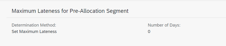
19. Maximum lateness allowed (Fixed orders – Deliveries)

One can model late less for fixed orders using below settings in planning run profile but you can also discuss with SAP to use the additional parameter from SAP to meet all the fixed order demand by exact number of days for late ness.

20. Transport Discount Factor

In some scenario, we have seen that if inventory holding cost is same at both location and we wanted to create stock transfer near to the demand for target location but due to same cost optimizer can create stock transfer earlier / latter which don’t create any cost difference. This scenario can be addressed by modelling Transport cost discount factor using key figure calculation where we can decease transport cost by X% in every bucket.

21. Product Decomposition

We have various settings available in planning run profile to solve deployment optimizer by Product de-composition method, it helps to improve performance and solve quality. Most of the time when we are not modelling any capacity constraint then we can solve every product as unique sub problem

22. Location Product Substitution (Limitations)

This feature is very similar to Time series location product substitution but overall limiting the ability to create transport during SOFTSTOP phase creates lot of challenge to use the existing stock of old product effectively. This basically gets locked to one particular location and cannot be moved during deployment.

23. Deployment orders getting generated on same day as of receipts

Currently there is no available feature in OBP by which we can control that any available/incoming receipt cannot be considered as available to deploy on the same day. To achieve the same, we have modelled Goods receipt processing time of 1 day at source location, this basically ensures that your receipt availability is delayed by one day and hence aligns properly with your deployment plan.

24. UOM Conversion

There is a technical limitation in OBP that we can’t apply UOM conversion to the key figures that are input to engine ex – Safety Stock, Forecast Unconstrained.

So, in case if your planner wants to see this data with different UOM’s you can create separate custom key figures which are enabled with UOM conversion and derived from standard.

25. Use of Planning Version

If we integrate transactional data multiple times in a day and due to that if we want to keep our base plan static or if we want to do any what-if simulation then use of planning version is very help. One needs to keep in mind below :

• Make relevant settings in setting for order-based planning app
• Copy Order related data into simulation version
• Copy TS KF into simulation version
• Taken deployment planning run at version level, if required

26. Discretization Horizon at source location

By default, SAP offers Discretization horizon to be considered by receiving location but with use of additional expert parameter its possible to consider this horizon at supply location too

27. IBP2308 change

Earlier Deployment optimiser, were evening considering the product location which were not part of planning filter selection but in IBP2308 SAP has brought the improvement to ignore any product location which are not connected by transportation lane.  This way its controlled that unnecessary product location are not selected during deployment run.

28. Switchable constraint

Using Switchable constraint, we can switch on / off some of the constraints to be used in deployment planning run. This setting is available in planning run profile and very useful.

Few of the noticeable switchable constraints are freeze horizon, capacity etc. We have used switchable constraint of freeze horizon (Freeze horizon = Yes and maintained as 99) very nicely to not let optimizer plan anything rather just calculate updated demand fulfilment numbers.

29. Planning Run Monitor

We have a separate blog on this topic, While its very complicated and uncomplete for OBP Optimizer it’s a very useful feature for TS Optimizer. It will still take some time for OBP planning run monitor to become simple and user friendly.

Conclusion – Deployment Optimizer is a useful feature in IBP OBP which can definitely be used if customers are looking for a planning engine for short term. There are definitely some useful features which comes with SAP standard however, the engine still needs some noticeable improvements.

Few of the improvements which we think are essential to make this functionality complete are :

• Storage and Handling Capacity
• Auto-update of priority in Deployment stock transfer (this is very useful feature if you are using TLB), this feature was available with SAP APO
• Interactive order creation in Planning view
• Defining ATD on Location or Location-Product level
• Supporting inspection lot and stock under quarantine
• BADI support (like APO) to write your own custom logic and modify data

About the Author :

Girish Kumar Jain is a Senior Solution Architect having more then 20+ years of experience in implementing SAP tools like IBP/APO. He has successfully lead and delivered large scale IT implementations projects for several Fortune 500 clients like Lion, CCEP, Unilever, Reckitt Benckiser etc

If you are interested to learn and explore more on SAP IBP then contact us on info@smartcons.nl